And we back. Welcome to Data Science Some Days. A series where I go through some of the things I’ve learned in the field of Data Science.
For those who are new… I write in Python, these aren’t tutorials, and I’m bad at this.
Regarding the title – I’m kidding, I haven’t been anywhere. I’m just bad at writing. However, I recently completed a Hackathon. Let’s talk about it.
Public Health Hackathon
This crept up on me (I forgot about it…). Given it was over the course of a weekend, it threw all the plans I didn’t have out of the window.
#Our task was to tackle a health problem with public datasets. Many of the datasets supplied were about Covid-19 and I really didn’t need to study it while living in my first pandemonium. Not having it.
So we picked air quality and respiratory illness instead. Why? Hell if I know. I think it was my idea too. However, there was a lot of data for the US so it proved helpful for us.
I think we started this problem backwards. We thought about how we’d like to present the information and then thought about what we wanted to do with the data. It wasn’t a problem, just peculiar on reflection.
We decided to present our information as a Streamlit dashboard. This, when it worked, was brilliant. We then did some exploratory data analysis, developed a time forecasting model and allowed people to see changes in respiratory conditions in the future.
Streamlit is a fast way to build and deploy web apps without needing to use a more complex framework or require front-end development experience.
This was probably the most useful part because I’ve been interested in trying out Streamlit for a while. It seems to a relatively powerful and I’m confident that the people behind it will continue to improve its functionality.
The main benefit for me was its fast feedback loop. As soon as you update your script, you can quickly refresh the application locally to see your changes. If you make an error, it shows it on screen rather than crashing.
The second benefit is its integration with popular data visualisation and manipulation packages. It’s easy to insert code from Pandas and Plotly without much change. It also contains native data visualisation functions which are helpful but not nearly as interactive as specialised packages.
The third benefit is that it’s a great way to deploy machine learning results to the public. One thing I’ve been stuck on in my Data Science journey is how to show findings to others without having to just share notebooks. Not everyone wants to read bad code.
I’ll likely want to go into more depth into Streamlit at some point. But not today. I like it though.
2. Working with others
The only other time I’ve worked collaboratively with code is in my first Hackathon!
It’s a valuable experience being able to quickly learn the strengths and weaknesses of your teammates, decide on a task and delegate. It’s as much of a challenge as it is fun – especially when you are fortunate enough to have good teammates.
We didn’t utilise git much though and it showed that version control through Google Drive becomes unweildy fast.
3. General practice
It’s always good to practice. I’m bad at coding, which will never change. But the aim is to become less bad. I think I became less bad as a result of the hackathon.
Other things…
I’m halfway through my second round of #66daysofdata started by Ken Jee and I’ve been more consistent than the previous attempt. Definitely taken advantage of the “minimum 5 minutes” rule! There have been many days where the best I’ve done is just watch a video.
At the moment, I’ve been learning data science and Python without much direction. Mainly trying to work on projects and quickly getting discouraged by things not working. For example, in my last post about working on more projects, I was working on a movie recommendation system. It failed at multiple points and eventually I stopped working on it. Then didn’t pick anything else up.
My next Data Science Some Days post will hopefully contain a structured learning plan. Unless I finish my movie recommendation system.
And we back. Welcome to Data Science Some Days. A series where I go through some of the things I’ve learned in the field of Data Science.
For those who are new… I write in Python, these aren’t tutorials, and I’m bad at this.
I haven’t written one of these for an entire month. My mistake… time flies when you procrastinate.
I want to spend a little bit of time talking about learning Data Science itself.
I won’t say how long I’ve been learning to code and such because I don’t really know the answer. This isn’t to say I’ve been doing it for a long time, I just don’t have much of a memory for this stuff.
I will, however, say one of the big mistakes I’ve made in my journey:
Not completing enough projects.
Any time I start a new project, I feel figuratively naked – as though all the knowledge I’ve ever gathered has deserted me and I’ll never be able to find it again.
I find it difficult to do anything at all until I get past the initial uncomfortable feeling of not having my hand held through to the end. Will I fall over? Yes. But learning how to get back up is a really useful skill, even if you fall over after another step.
There are a lot of tutorials online about all sorts of things. Many of them are good, some are bad, some are brilliant. When it comes to programming, you will never have a shortage of materials for beginners. As a result, they’re tempting and the entry point is quite low. Many even have no idea where to start.
Tutorials are also easy to get lost in because they do a lot of the heavy lifting in the background. That’s the more helpful way to teach information but perhaps less useful for the learner. This isn’t to say all tutorials and courses are “easy”. Far from it. Rather, no one has ever become a developer or programmer purely off the back of completing a handful of tutorials.
Don’t get attached to tutorials or courses. They can only take us so far. It’s also difficult to stay entertained by them for the long haul.
This divorces you quite quickly from an attachment to completing courses or selecting the “right one”. If you’ve got what you need out of it, then move on and use the knowledge to create something. Fortunately, the information doesn’t disappear if you tell yourself you might not complete it. It’s fine to refer to them during projects, anyway.
You’ll get to the difficult parts more quickly which lets you understand the true gaps in your knowledge/skill. It’s perfectly fine for this to be humbling. Getting better at anything requires humility.
It’s more fun
Being the person responsible for creating something is a really satisfying feeling, even if it sucks. (It likely does, only in comparison to those who are much more experienced than you, which is unfair. Comparison is a fools game.)
You can point to a model you’ve trained or visualisation you’ve created and say “That was ME”. And it’ll be true.
When you look at a list of potential projects, you’re more likely to add your own twist to it (it doesn’t matter if that’s just experimenting with different colours). If you’re following a tutorial to the T, you miss out on something important:
Ownership.
The difficulties and successes are yours.
Leave yourself open to surprises
I’ve noticed a few things in a recent project of mine (more on that in the next DS Somedays post, it’s nothing special):
I know and understand a bit more than I gave myself credit for
There is so much more I can add to my knowledge base to improve the project
Courses, tutorials, tools are just there to help me reach my end goal. It helps explain why I always have so many tabs open
They can be challenging, which might also explain why they’re easy to avoid. However, I’ll definitely have to work towards doing more. If not for my portfolio but general enjoyment.
And we back. Welcome to Data Science Some Days. A series where I go through some of the things I’ve learned in the field of Data Science.
For those who are new… I write in Python, these aren’t tutorials, and I’m bad at this.
When I’m cooking, sometimes I’m too nervous to taste the food as I’m going along. It’s like, I must think that I’m being judged by my guests over my shoulder.
That’s a rubbish approach because I might reach the end and not realise that I’ve missed some important seasoning.
So, if you want a good dinner, it’s important you just check as you’re going along.
This analogy doesn’t quite work with what I’m about to explain but I’ve committed. It’s staying.
Cross-Validation
The first introduction to testing is usually just an 80/20 split. This is where you take 80% of your training data and use that to train your model. The final 20% is used for validation. It comes in the following form:
X = training_data
y = training_data["prediciton target"]

X_train, X_valid, y_train, y_valid = train_test_split(X,y,train_size=0.8,test_size=0.2)
This is fine for large data sets because the 20% you’re using to test your model against will be large enough to offset the random chance that you’ve just managed to pick a “good 20%”.
With small data sets (such as the one from the Housing Prices competition from Kaggle), you could just get lucky with your test split. This is where cross validation comes into play.
This means you test your model against multiple different subsets of your data. It just takes longer to run (because you’re testing your model many different times).
It looks like this instead:
# cross_val_score comes from sklean.model_selection.
# The pipeline here just contains my model and the different things I've done to clean up the data
# You multiply by -1 because sklearn uses "higher number is better" and this allows consistency

scores = -1 * cross_val_score(my_pipeline, X, y,
                              cv=5,
                              scoring='neg_mean_absolute_error')
“cv=5” determines the number of subsets (or better known as “folds”).
The more you use, the smaller the amount of data you use per test. It might take longer but with small data sets, the difference is negligible.
It’ll spit out a list of scores, then you can just average it to get the best model.
I heard the test results were positive.
Conclusion
Cross validation is a helpful way to test your models. It helps reduce the chance that you simply got lucky with the validation portion of your data.
With larger data sets, this is less likely though.
It’s important to keep in mind that cross validation increases the run time of your code because it runs your model multiple times (one on each fold for example).
Also, I’m aware that my comic doesn’t make that much sense but it made me laugh so I’m keeping it.
And we back. Welcome to Data Science Some Days. A series where I go through some of the things I’ve learned in the field of Data Science.
For those who are new… I write in Python, these aren’t tutorials, and I’m bad at this.
Today, we’re going to go talk about Pipelines – a tool that seems remarkably helpful in reducing the amount of code needed to achieve an end result.
Why pipelines?
When creating a basic model, you need a few things:
Exploratory Data Analysis
Data cleaning and sorting
Predictions
Testing
Return to number one or two and repeat.
As you make different decisions with your data, the more complex the information, the easier it might be to miss a step or simply forget the steps you’ve made! My first model involved so many random bits of code. If I had to reread it, I’d have no idea what I wanted to do. That’s even with comments.
Pipelines help combine different steps into smaller amounts of code so it’s easier. Let’s take a look at what this might look like.
The data we have to work with
As we may know, the data we work with might have many different types of data. Within the columns, they may also have missing values everywhere. From the previous post, we learned that’s a no go. We need to fill in our data with something.
We have numbers (int64) and strings (object – not strictly just strings but we’ll work with this).
So we know that we have to fill in the values for 3 of the 4 columns we have. Additionally, we have to do this for different kinds of data. We can utilise a Simple Imputation and OneHotEncoder to do this. Let’s try to do this in as few steps as possible.
Creating a pipeline
#fills missing values with the mean across the column when applied to dataset
numerical_transformer = SimpleImputer(strategy="mean")

# replaces the categorical columns with a number (1 for yes, 0 for no) when applied to dataset
categorical_transformer = Pipeline(steps=[
    ('imputer', SimpleImputer(strategy='constant')),
    ('onehot', OneHotEncoder(handle_unknown='ignore'))])

# Let's apply the above steps using a "column transformer". A very helpful tool when
preprocesser = ColumnTransformer(transformers=[("num", numerical_transformer, numerical_columns),
("cat", categorical_transformer, categorical_columns)])
Ok, we’ve done a lot here. We’ve defined the methods we want to use to fill in missing values and how we’re going to handle categorical variables.
Just to prevent confusion, “ColumnTransformer” can be imported from “sklearn.compose”.
Now we know that the methods we are using are consistent for the entirety of the dataset. If we want to change this, it’ll be easier to find and simpler to change.
Then we can put this all into a pipeline which contains the model we wish to work with:
# bundles the above into a pipeline containing a model
pipeline_model = Pipeline(steps=[('preprocessor', preprocessor),
                      ('classifier', RandomForestClassifier())])
This uses a small amount of code. So now we can use this when fitting our model to the training data we have then later making predictions. This is instead of trying to make sure our tables are all clean and accidentally applying predictions to the wrong table (I have done this…), we can just send the raw data through this pipeline and we’ll be left with a prediction.
Pipelines have been an interesting introduction to my Data Science journey and I hope this helps give a rough idea of what they are and why they might be useful.
Of course, they can (and will) become more complex if you are faced with more difficult problems. You might want to apply different methods of filling in missing values to different sections of the data set. You might want to test multiple different models. You might want to delete Python from your computer because you keep getting random errors.
Whatever it may be, just keep trying, and experimenting.
I’m going through the Kaggle Intermediate Machine Learning course again to make sure that I understand the material as I remember feeling a bit lost when I started on a different project.
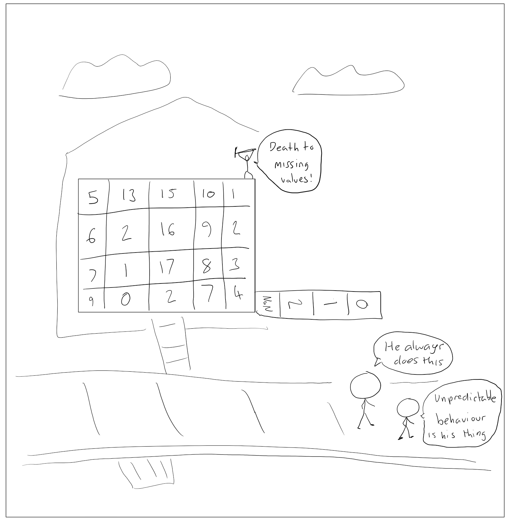
Here are some things that I’ve gone over again from the “Missing Values” section of the course.
Introduction
In machine learning, we do not like missing values. They make the code uncomfortable and it refuses to work. In this case, a missing value is “NaN”. A missing value isn’t “0”. Imagine an empty cell rather than “0”. If we don’t know anything about a value when we can’t use it to make a prediction.
As a result, there are a few techniques we can use when playing around with our data to remove missing values. We can do that by getting rid of the column completely (including the rows _with_ information), filling in the missing values with a certain strategy, and filling in missing values but making sure we say which ones we’ve filled in.
Another final note before those who haven’t come across this series before – I write in Python, I tell bad jokes and I’m not good at this.
The techniques
First, let’s simply find the columns with missing values:
missing_columns = [x for x in training_data[x] if train_columns[x].isnull().isna()]
This uses List Comprehension – it’s great. I’d use that link to wrap your head around it (if you haven’t).
In the Kaggle course, it uses a Mean Absolute Error method of testing how good a prediction is. In short, if you have a prediction and data you know is correct… how far away is your prediction from the true value? The closer to 0 the better (in most cases. I suppose it may not be that helpful if you think you’re overfitting your data).
Dropping values
If we come across a column with a missing value, we can opt to drop it completely.
In this case, we may end up missing out on a lot of information. For example, I have a column with ten thousand rows and 100 are NaN, then I can no longer use over 9 thousand pieces of information!
This uses a function called “Simple Imputation” – the act of replacing missing values by inferring information from the values you do have.
You can take the average of the values (mean, median etc) and just fill in all of the missing values with that information. It isn’t perfect, but nothing is. We can do this using the following:
So if you’re a bit confused as to why we use “.fit_transform()” on the training set but only “transform()” on the validation set, here is why:
“fit_transform()” performs two actions in one line. It “fits” the data by calculating the mean and variance of the training set. It then transforms the rest of the features using that mean and variance information. We are training the model.
We don’t want to do “fit” the validation data because the prediction is made based on what has been learned from the training set. The data set is different and we want to know how well the model performs when faces with new information.
This method performs better than just dropping values and it is possible to play around with the method in imputation. The default is replacing the values with the mean but it’s worthwhile playing around and seeing what gives you better results.
It’s also important to note that this only works with numerical information! Why? A lot of data sets have missing labels. For example, if you had the colour of a house in your data set, trying to get the mean of green and orange is impossible (it’s also ugly).
The end
There are many other methods with different pros and cons (there’s forward filling and backward filling which I won’t go into detail here) but I want to keep this post relatively short.
This is were bias and mistakes begin to creep into the model because we are always making decisions about what to do with the information that we have. That’s important to keep on mind as they become more complex.
Firstly, the title is a joke. I really have no helpful insights to share as you’ll see from my work.
This will be split into a few sections
What is machine learning?
Train and test data
Visualising the training data
Creating a feature
Cleaning the data
Converting the data
Testing predictions with the test data
Final thoughts
It should definitely be mentioned that this is the furthest thing from a tutorial you will ever witness. I’m not writing to teach but to learn and tell bad jokes.
One of the basic tasks in machine learning is classification. You want to predict something as either “A will happen” or “B will happen”. You can do this with historical data and selecting algorithms that are best fit for purpose.
The problem we are posed with is:
Knowing from a training set of samples listing passengers who survived or did not survive the Titanic disaster, can our model determine based on a given test dataset not containing the survival information, if these passengers in the test dataset survived or not.
Kaggle – Machine Learning From Disaster
2. Train and Test data
Kaggle, the data science website, has a beginner problem called “Titanic – Machine Learning from Disaster” where you’re given data about who survives the titanic crash with information about their age, name, number of siblings and so on. You’re then asked to predict the outcome for 400 people.
The original table looks something like this:
PassengerId
Survived
Pclass
Name
Sex
Age
SibSp
Parch
Ticket
Fare
Cabin
Embarked
1
0
3
Braund, Mr. Owen Harris
male
22.0
1
0
A/5 21171
7.2500
NaN
S
S
2
1
1
Cumings, Mrs. John Bradley (Florence Briggs Th…
female
38.0
1
0
PC 17599
71.2833
C85
C
C
3
1
3
Heikkinen, Miss. Laina
female
26.0
0
0
STON/O2. 3101282
7.9250
NaN
S
S
4
1
1
Futrelle, Mrs. Jacques Heath (Lily May Peel)
female
35.0
1
0
113803
53.1000
C123
S
S
5
0
3
Allen, Mr. William Henry
male
35.0
0
0
373450
8.0500
NaN
S
S
Initial table for titanic problem
This is what we call “training data”. It is information that we know the outcome for and we can use this to make our fit our algorithms to then make a prediction.
There is also “test” data. It is similar to the data above but with the survived column removed. We will use this to check our predictions against and see how well our efforts have done with all of the visualisations and algorithm abuse we’re doing.
3. Visualising the data
To start with, it’s important to simply have a look at the data to see what insights we can gather from a birds eye view. Otherwise we’re just staring at tables and then hoping for the best.
Information as a histogramInformation as a box plot
I won’t go through everything (and yes, it is very rough) but we can gain some basic insights from this. It might influence whether we want to create any new features or focus on certain features when trying to predict survival rates.
For example, we can see from the box plots that most people were roughly 30 years old and had one sibling on board (2nd row, first two box plots). From the histograms, we can see that most people were in passenger class 3 (we have no idea what that means in real life) and a lot of people on the titanic (at least in this dataset) were pretty young.
How does this impact survival? I’m glad you asked. Let’s look at some more graphs.
Survival rates vs passenger class, sex and embarking location. Women in passenger class 1 seemed to live…
Women seemed to have a much higher chance of survival at first glance
Now, we could just make predictions based off these factors if we really wanted to. However, we can also create features based on the information that we have. This is called feature engineering.
4. Creating a feature
I know, this seems like I’m playing God with data. In part, that is why I’m doing this. To feel something.
We have their names with their titles includes. We can extract their titles and create a feature called “Title”. With this, we’ll also be able to make a distinction between whether people with fancy titles were saved first or married women and so on.
for dataset in new_combined:
    dataset['Title'] = dataset.Name.str.extract(' ([A-Za-z]+)\.', expand=False)
You don’t need to understand everything or the variables here. They are specific to the code written which is found on my GitHub.
It basically takes the name “Braund, Mr. Owen Harris” and finds a pattern of the kind A-Za-z with a dot at the end. When this code is run, it’ll take out “Mr.” because it fits that pattern. If it was written as “mr” then the code would miss the title and ignore the name. It’s great, I’ll definitely be using the str.extract feature again.
5. Cleaning the data
A lot of data is bad. Data can regularly contain missing values, mistakes or simply be remarkably unhelpful for our goals. I’ve been told that this is large part of the workflow when trying to solve problems that require prediction.
We can get this information pretty quickly:
new_combined.info() #This tells us all the non-null values in the data set
new_combined.isna().sum() #This tells us which rows have null values (it's quicker then the first method)
In the titanic data set, we have loads of missing data in the “age” column and a small amount in the “embarked” column.
For the “age” section, I followed the advice from the tutorial linked above and guessed the ages based on their passenger class, and sex.
For the “embarked” section, because there were so few missing values, I filled them in using the most common location someone embarked on.
As you can see, cleaning data requires some assumptions to be made and can utilise different techniques. It is definitely something to keep in mind as datasets get bigger and messier. The dataset I’m working with is actually pretty good which is likely a luxury.
It isn’t sexy but important. I suppose that’s the case with many things in life.
5. Converting the data
In order for this information to be useful to an algorithm, we need to make sure that he information we have in our table is numerical.
We can do this by mapping groups of information to numbers. I did this for all features.
It basically follows this format:
for item in new_combined:
    item.Sex = item.Sex.map({"male":0, "female":1}).astype(int)
It is important to note that this only works if all of the info is filled in (which is why the previous step is so important).
For features that have a large number of entries (for example, “age” could potentially have 891 unique values), we can group them together so we have a smaller number of numerical values. This is the same for “fare” and the “title” feature created earlier.
It is basically the same as above but there is one prior step – creating the bands! It is simply using the “pd.cut()” feature. This segments whichever column we specify into the number of bands we want. Then we use those bands and say something like:
“If this passenger is between the age of 0 and 16, we’ll assign them a “1”.”
Our final table will look like this:
Survived
Pclass
Sex
Age
SibSp
Parch
Fare
Embarked
Title
0
3
0
1
1
0
0.0
1
3
1
1
1
2
1
0
3.0
3
4
1
3
1
1
0
0
1.0
1
2
1
1
1
2
1
0
3.0
1
4
0
3
0
2
0
0
1.0
1
3
Much less interesting to look at but more useful for our next step
6. Testing predictions with the test data
Now we have a table prepared for our predictions, we can select algorithms, fit them to our training data, then make a prediction.
While the previous stages were definitely frustrating to wrap my head around, this section certainly exposed just how much more there is to learn! Exciting but somewhat demoralising.
There are multiple models you can use to create predictions and there are also multiple ways to test whether what you have done is accurate.
So again, this is not a tutorial. Just an expose of my poor ability.
Funnily enough, I also think this is where it went wrong. My predictions don’t really make any sense.
To set the scene – we have:
A table of features we’ll use to make a prediction (the above table) = X
A prediction target (the “survived” column) = y
We can split our data into 4 sections and it looks like so:
train_X, val_X, train_y, val_y = train_test_split(X, y, random_state = 0)
This splits our data into the four variables I’ve specified. “Random_state = 0” just means we get the same data split every time the script is run (so randomised data splits is false).
Now we can define our models. I picked a variety of different models to see what results I would get and will hopefully be able to explain the models in another post. However, a detailed understanding of them isn’t necessary at the moment.
I used two linear models and four non-linear models. The most accurate model I used was “SVC” or Support Vector Classification.
SVM = SVC(gamma='auto')
 #Defines the model

SVM.fit(train_X.drop(["Survived"],axis=1), train_y) #Allows the model to "learn" from the data we have provided

Y_prediction = SVM.predict(test_X.drop(["PassengerId"], axis=1)) #predicts the values that should be in the "survived" column

acc_log = round(SVM.score(train_X.drop(["Survived"],axis=1), train_y) * 100, 2)
 # Returns the mean accuracy based on the labels provided

acc_log # returns the accuracy as a percentage
My final result was 83.7% accuracy!
My first attempt led me to a 99.7% accuracy – Ain’t no way! And the kicker? It predicted everyone would die!
I did this entire project for this comic.
At this point, my brain rightfully died and I submitted my prediction to the Kaggle competition with it being better than 77% of other users. So there is much room for improvement.
8. Final thoughts
This is a beginner problem designed to help people get used to the basics of machine learning so the dataset is better than you’d usually get in the real world.
As I was working through this, I noticed that there are a lot of decisions we can make when creating a prediction. It sounds obvious but it’s important. This is where normal cognitive biases creep in which can go unnoticed – especially when the information we’re working with is far more complex and less complete.
For example, if any of the features were less complete, our decisions on how to fill them in would make a greater impact on our decisions. The algorithms we choose are never a one size fits all solution (which is why we often test many).
I’ll publish my code on my GitHub page when I’ve cleaned it up slightly and removed the swear words.
I’ve probably made a really dumb mistake somewhere so if you feel like looking at the code, please do let me know what that might be…
And with that, I bring it to an end.
There will be much more to improve and learn but I’m glad I’ve given this a shot.
My honourable guests, thank you for joining me today to learn how to copy the entire internet and store it in a less efficient format.
A recent project of mine is working on the Police Rewired Hackathon which asks us to think of ways to address hate speech online. Along with three colleagues, we started hacking the internet to put an end to hate speech online.
We won the Hackathon and all of us were given ownership of Google as a reward. Google is ours.
Thank you for reading and accepting your new digital overlords.
Our idea is simple and I will explain it without code because my code is often terrible and I’ve been saved by Sam, our python whisperer, on many occasions.
Select a few twitter users (UCL academics in this case)
Take their statuses and replies to those statuses
Analyse the replies and classify them as hate speech, offensive speech, or neither
Visualise our results and see if there are any trends.
In this post, I will only go through the first two.
Taking information from twitter
This is the part of the hackathon I’ve been most involved in because I’ve never created a Twitter scraper before (a program that takes information from Twitter and stores it in a spreadsheet or database). It was a good chance to learn.
For the next part to make sense, here’s a very small background of what a “tweet” is.
It is a message/status on Twitter. With limited amounts of text – you can also attach images. These tweets contain a lot of information which can be used to form all sorts of analysis on. For example, a single tweet contains:
Text
Coordinates of where it was posted (if geolocation is enabled)
the platform it came from (“Twitter for iPhone”)
Likes (and who liked them)
Retweets (and who did this)
Time it was posted
And so on. With thousands of tweets, you can extract a number of potential trends and this is what we are trying to do. Does hate speech come from a specific area in the world?
OK, now how do we get this information?
There are two main ways to do this. The first is by using the Twitter Application Programming Interface (API). In short, Twitter has created this book of code which people like me can interact with with my code and it’ll give me information. For example, every tweet as a “status ID” that I can use to differentiate between tweets.
All you need to do is apply for developer status and you’ll be given authentication keys. There is a large limitation though – it’s owned by Twitter and Twitter, like most private companies, value making money.
There is a free developer status but that only allows for a small sample of tweets to be collected up to 7 days in the past. Anything beyond that, I’ll receive no information. I also can’t interact with the API too often before it tells me to shut up.
Collecting thousands of tweets at a decent rate would cost a lot of money (which people like myself… and most academics, cannot afford).
Fine.
Programmers are quite persistent. There are helpful Python modules (a bunch of code that helps you write other code) such as Twint.
Twint is a wonderfully comprehensive module that allows for significant historical analysis of Twitter. It uses a lot of the information that Twitter provides, does what the API does but without the artificial limitations from Twitter. However, it is fickle – for an entire month it was broken because twitter changed a URL.
Not sustainable.
Because I don’t want to incriminate myself, I will persist with the idea that I used the Twitter API.
How does it work?
Ok, I said no code but I lied. I didn’t know how else to explain it.
for user in users:
    tweets_pulled = dict()
    replies=[]
    for user_tweets in tweepy.Cursor(api.user_timeline,screen_name=user).items(20):
        for tweet in tweepy.Cursor(api.search,q='to:'+user, result_type='recent').items(100): # process up to 100 replies (limit per hour)
            if hasattr(tweet, 'in_reply_to_status_id_str'):
                if (tweet.in_reply_to_status_id_str==user_tweets.id_str):
                    replies.append(tweet)
I’ve removed some stuff to make it slightly easier to read. However, it is a simple “for loop”. This takes a user (“ImprovingSlowly”) and takes 20 tweets from their timeline.
After it has a list of these tweets, it searches twitter for “ImprovingSlowly” and adds to a list whether the tweets found were replies to any statuses.
Do that for 50 users with many tweets each, you’ll find yourself with a nice number of tweets.
If we ignore the hundred errors I received, multiple expletives at 11pm, and the three times I slammed my computer shut because life is meaningless, the code was pretty simple all things considered. It helped us on our way to addressing the problem of hate speech on Twitter.
Limitations
So there are many limitations to this approach. Here are some of the biggest:
With hundreds of thousands of tweets, this is slow. Especially with the limits placed on us by Twitter, it can take hours to barely scratch the surface
You have to “catch” the hate speech. If hate speech is caught and deleted before I run the code, I have no evidence it ever existed.
…We didn’t find much hate speech. Of course this is good. But a thousand “lol” replies doesn’t really do much for a hackathon on hate speech.
Then there’s the bloody idea of “what even is hate speech?”
I’m not answering that in this blog post. I probably never will.
Conclusion
Don’t be mean to people on Twitter.
I don’t know who you are. I don’t know what you want. If you are looking for retweets, I can tell you I don’t have any to give, but what I do have are a very particular set of skills.
Skills I have acquired over a very short Hackathon.
Skills that make me a nightmare for people like you.
If you stop spreading hate, that’ll be the end of it. I will not look for you, I will not pursue you, but if you don’t, I will look for you, I will find you and I will visualise your hate speech on a Tableau graph.
While George Floyd was being killed, he called for his mum.
I can’t move Mama Mama
His mum had passed away two years prior to this moment yet, at the forefront of his memory as he understands he could die, he calls for her. He is not delirious, dumb or silly. He knew what he was doing and why.
In that moment, he simply wanted his mum.
When I call for my mum, I call for the woman who stayed with me for 100 days while I was in an incubator in the early days of my life.
When I call for my mum, I call for the woman who would go to work in the early hours of the morning, come back late, and still want to know what my day was like in school.
When I call for my mum, I call for the woman who wanted the best for her children every day and tried to make sure it happened.
When I call for my mum, I call for the woman who wishes she could take my chronic pain and hold it herself just to make sure that I’m comfortable.
When I call for my mum, I find myself calling for warmth, love, and fantastic jollof rice with plantain (mum, if you’re reading this – please and thank you).
I’m lucky to have wonderful women in my life who are still here to experience its ups and downs with me. For that, I will be thankful.
I am lucky I am able to be thankful because my life wasn’t slowly squeezed out of my body at the hands of someone who was meant to protect me.
In the midst of these protests, this anger, this injustice, let us remember that the community we are fortunate to have, will often carry us through adversity. Sometimes how we approach adversity will change the world. Other times, it’ll change our small knit community. Maybe it’ll even just change one mind.
Often, the smallest changes that are made consistently over time will be the most impactful ones. Attitudes, thoughts and feelings will change. To help the world finally understand what it means for a black life to matter.
Gianna Floyd now says “Daddy changed the world!”
Indeed he has, Gianna. He will continue to do so.
For me, my world has been strongly influenced by my mum, my grandmother and aunts. For my dad, I know his world has been influenced by his mum.
In these times, I think of all of the black men and women who have been unjustly killed as a result of systematic racism. How many of them thought of their mum’s in their last moments?
Perhaps, when the world cries for its mum, it cries for love and warmth too. Or even the anger that only mothers seem to have when their child is hurt.
Last year I did a reading challenge. I wanted to hit 40 books read for the year and was recording my progress on Goodreads.
I promptly forgot to log anything on Goodreads for the entire year, tried to remember what I read throughout the year and hoped that I remembered everything.
I didn’t. I got mixed up with books that I read in 2016 so I have no idea how many books I read last year.
In 2020, I’ve realised that doesn’t matter at all. WHO CARES if someone has read a book a week for the entire year…
Instead, I’d like to increase the amount of time spent reading rather than the number of books read.
Using the number of books and a measuring metric encourages skimming, and picking shorter books to stay on track.
Trying to maximise the amount of time spent reading accomplishes the whole point of these reading challenges. To read more – without making you feel bad for being “slow” or “reading short books” or “lying about the number of books read”.
I’ve said my piece… onto the good stuff.
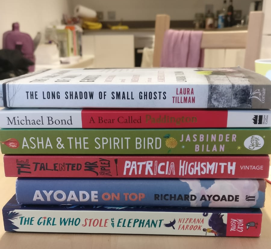
Books I read in January
The Long Shadow of Small Ghosts – Laura Tillman
An insightful read that has evidently been treated with the appropriate sensitivity required of a case like this. She managed to bring in the impact the case had on a small community through valuable interviews and research.
Unfortunately, overall, it wasn’t all that interesting.
When I finished the book, I genuinely felt that her talents were wasted on this case. She has the ability to navigate sensitive areas well but my goodness, the case, while gruesome, just failed to interest me. Pity.
The Girl Who Stole An Elephant – Nizrana Farook
A very enjoyable and easy read (and I was disappointed it was over!) The characters were a pleasure to know as their friendship grew during their journey.
Apparently, stealing an elephant will force you to become well acquainted.
I picked this up because I loved the cover and I’ve been enjoying children’s books a lot. This didn’t disappoint – though the ending was slightly rushed.
Ayoade On Top – Richard Ayoade
This was a short, enjoyable read about, yes, a film no one has seen. Including me. However, this has convinced me to fill the aeroplanecentric-comedy-hole in my heart.
Ayoade’s personality shines through every page and it’s wonderful that it isn’t just another biography.
I still haven’t watched the film yet though, so my opinions may change after the viewing…
The Talented Mr Ripley – Patricia Highsmith
This book is a wonderful thriller and I haven’t read one of this sort in a while.
The main shortcoming is that it’s only in the second half of the book do we understand just how talented Mr Ripley is… And how much luck he has on his side.
But the ending was a masterclass in tension building. Brilliant!
Really enjoyed this read – mainly surprised I hadn’t read it sooner!
A Bear Called Paddington – Michael Bond
Everyone has heard of Paddington but I realised I had never read the books. Without a doubt, one of the most fun books I have ever read.
Paddington, a bear from the darkest Peru always gets himself into some kind of commotion but despite his best intentions. … But let’s not forget, he is a literal bear.
We can’t blame him for too much, can we?
Ladies and gentlemen, 2020 may have only just started but this may be my book of the year. I decided that, during lunch and my afternoon walk, I’d go to Waterstones, sit down and read a chapter.
The perfect cure to a bad day. I recently watched the film too – wonderful adaptation. I love Paddington, I love the Brown family, I love Mr Gruber, I love everything about Paddington Bear.
And that brings me to the end.
The number of books may be unsustainable for the year but I will do my best to maintain or increase the amount of time I spend reading.
Ladies and gentlemen, this has been a long time coming.
So, I’ve finally started programming. Technically, I started months ago but I’ve made such a piss-poor effort at being consistent, that I’ve done next to nothing.
I was growing frustrated – often having nightmaresasking the question – will I ever be able to say “Hello World”?
Evidently, simply thinking about it would never work. I can buy as many Udemy courses as I want – that won’t turn me into a data scientist. My wonderful solution to this is to go straight into a project and learn as I go. I’m learning python 3.6. But first…
print("Hello World")
I have joined the elites.
Ok, the project goes as follows:
I need to send emails to specific groups of people a week before the event starts. The email should also include attachments specific to the person I’m sending the email to and it will have HTML elements to it.
To break it down…
I need to send an email
I need to send a HTML email
I need to send a HTML email with attachments
I need to send a HTML email with attachments to certain people
There’s more but I’ve only managed the first two so far. This programming stuff is difficult and the only reason why I’m not computer illiterate is because I was born in the 90s.
They’re both great and use slightly different methods to achieve the same result. Maybe you’ll notice that my final solution ends up being a desperate cry for help combination of them both.
LET US BEGIN.
Here is the first iteration of the code:
import smtplib

#sets up simple mail transer protocol
smtpObj = smtplib.SMTP('smtp-mail.outlook.com', 587)

type(smtpObj)

#Connects to the outlok SMTP server
smtpObj.ehlo()

#Says "hello" to the server
smtpObj.starttls()

#Puts SMTP connection in TLS mode.

#I didn't get any confirmation when I ran the program though...
smtpObj.login('email1@email.com', input("Please enter password: ")

#Calls an argument to log into the server and input password.
smtpObj.sendmail('email1@email.com', 'email2@gmail.com', 'Subject: Hello mate \nLet\'s hope you get this mail')

#Email it's coming from, email it's going to, the message
smtpObj.quit()

#ends the session
print('Session ended')

#Tells me in the terminal it's now complete
Boom, pretty simple right? I mainly took everything from Automate the Boring stuff and just swapped in my details. Well, of course not. I kept on getting an error – nothing was happening.
Well – I was somehow using the WRONG EMAIL. FUCK. It took me an hour to realise that.
Next step… let’s send an email with bold and italics.
This was frustrating because nothing worked. All it really requires is for you to put in the message in HTML format. Because I’m not learning HTML, I decided to just use this nifty HTML converter to make this part less painful.
Here are my errors…
#regularly get "Syntax error" with smtpObj.sendmail - I was missing a fucking bracket
This literally made me to go bed angry.
'''everything in the HTML goes into the subject line -

smtpObj.sendmail('email@email', 'email2@gmail.com', "Subject: " f"Hello mate \n {html}")'''
This was a surprise but I figured out to stop it…
'''Now nothing shows up in the body of the message:

smtpObj.sendmail('email1@.ac.uk', 'email2@gmail.com', f"Subject: \n Hello mate {html}")

Solved by putting {html} next to \n'''
…then it somehow got worse…
'''Now... the email doesn't actually show up in html format

smtpObj.sendmail('email1@.ac.uk', 'email2@gmail.com', f"Subject: Hello mate\n{html}")'''
…and even worse.
At this point, I changed tactic and, in the process, the entirety of my code. I won’t show you everything here otherwise this post will look too technical to those who have no experience with coding but I’ve uploaded my progress so far onto Github.
To summarise, rather than trying to send HTML with the technique I used earlier, I used a module that was essentially created to make sending emails with python much easier (email.mime). This essentially means, it contains prewritten code that you can then use to create other programs.
But… I was successful in sending myself a HTML email. Now the next step is to add a bloody attachment without putting my head through my computer.
Dear reader, you may be wondering, “why is he putting himself through so much suffering? He sounds incredibly angry.
I’m not, I promise. This has actually been the most fun I’ve had in my free time in a while. It was a good challenge and I could sense myself improving after every mistake.
Granted, I probably should have just completed an online course or something before trying to jump into this project but that would have been less fun.